Filters are kinda sorta great…
What’s the first thing I do whenever I open a new spreadsheet? I filter it. Why? Because filtering is a great way to quickly analyze your data. Need to see which columns are and aren’t populated? Filtering is for you. Have users who don’t like to enter the same value, the same way twice? Use a filter to locate the inconsistencies.
You may have used Sorts to handle similar scenarios, but filters give you more control. Using them, you can also avoid having to constantly rearrange the rows of your data, lowering the odds of making a mistake.
What cool things can you do with filters?
- Say Goodbye to Empty Columns – A column with no data in it is a column you don’t need to import. I like a lean import file, and that means removing the clutter of blank columns.
- Spot a Bad Date or Phone – Filtering is a great way to quickly spot bad or missing dates, which can cause those pesky import errors. It can also clue you in to phone numbers that are inconsistently formatted.
- Make Sure It’s the Right List You’re Picking – Picklists in Salesforce are not very forgiving. It may be a small dot, but “Jr” and “Jr.” are not the same suffix. Filters can help you see those data vagaries. Then, a Find and Replace will equal a sparkly clean picklist.
- Work the Combinations – Filters are also a great way to check consistency across columns, for example, to check the data integrity of dependent picklists. If I’ve got a foundation type field, I can filter out the blanks in that column to verify all the records have a value of “Foundation” in the account type column. Or, in a donations table, I can check that all of the rows with a credit card type value, have “Credit Card” listed as the payment method.
- Use a Smarter Copy/Paste – This is a little more advanced, but I’ll often use filters to pull subsets of data that need to be imported separately such as when I’ve got spouse names in the same row as primary contacts. When you filter a set of columns and copy all, Excel grabs only those rows that meet the filtering criteria. Filtering out blank values for a spouse first name column, I can paste all of my spouse data to a separate tab for data prep.
I love filtering, but every operation in Excel has its gotchas and filters are no exception. One that’s gotten me is forgetting a filter is on when copying down a value to the rows beneath. That can overwrite values you don’t want to change, and unexpected data loss can lead to premature hair loss. Thank goodness there’s an undo button.
The mighty IF…
How powerful is a simple IF? It’s been said that any program can be written with only IF statements. I wouldn’t try that at home, but I do give the IF my unconditional endorsement for exquisitely handling many of the data manipulation scenarios I encounter. Need some proof? By writing an Excel formula that includes an IF (or a few, nested or strung together with an “&”) you can:
-
- Combine Multiple Lines of an Address – Many databases store street addresses as multiple lines of text, but not Salesforce. When you import addresses to Accounts and Contacts, you’re going to need to combine those fields into one block of text. This combination of two IFs will get that done.
- Set up Multi-Select Lists – One scenario I see a lot is the need to convert a series of True/False values or separate text strings into a single multi-select picklist. A set of IFs that concatenate strings and the “;” delimiter works wonders.
- Assign the Preferred Phone and Email – Most often, you won’t have an indicator in your table for which phones and emails are “preferred,” but the NPSP has a validation rule that requires you specify one (you can of course also turn the validation off). If you’ve got a hierarchy you’d like to enforce for when to use which phone, you can use a nested IF to assign the preferred phone type.
If you’ve ever worked with the Salesforce Formula Editor, the functionality in Excel is very much the same, although the syntax is different. Here, as you’ll see from the images, the syntax is =IF(logical test, value if true, value if false). Not so in the first example, I used a function CHAR(10). This adds a linebreak, which won’t be visible in the spreadsheet, but will show up in Salesforce when you import the value.
Dupes Making You See Red? Turn Them Pink
Do you have a sneaking suspicion that you’ve got a duplicate problem? Sometimes duplicate records are very obvious, but often times they’re well hidden. You can blush them out of hiding by using a handy little feature called Conditional Formatting.
By highlighting the cells in pink that have duplicate values in a column, you can easily visualize where the dupes are. You can even sort based on cell color to bring them to the top of the list. This is especially useful for quickly finding Contact records that have slightly different names but the same phone or email.
CRM Fusion’s Demand Tools offers a much more powerful tool for finding duplicates once they’re in your Salesforce, but if you want to assess the situation before the data is imported, this is a quick way to see the scope of the problem.
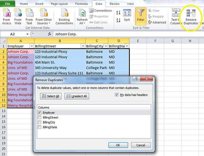
When there’s no doubt you’ve got duplicates, or cases where you need to create a unique list from a set of values, there’s a much more blunt instrument: Remove Duplicates. It’s a button on the Data tab. You can select one or more columns to use in identifying the duplicates. Excel will delete all duplicate values, keeping the first unique row for each repetition.
Let’s say you have a list of employer’s names for your contacts that you want to create affiliations for. You’re going to need to generate a unique list of the organization names to import as accounts. This is a perfect situation to use Remove Duplicates.
Filter out all of the blank values in the employer column, copy that column (and any others you want to import, such as work phone and address) to a separate tab, and then Remove Duplicates to create your import list. You can specify one or more columns for Excel to use in determining what’s a duplicate.
How will you link those imported names back to the contact’s records for the affiliations import? Funny you should ask, scroll down a little.
When Things are Looking Up…
Saving the best and most advanced for last, my final tip is the function called VLOOKUP. It’s not for the data meek but with its power, you won’t stay meek long.
Got a set of codes but you need to import a name or description instead? VLOOKUP can fix that. Want to add IDs to that list of unique orgs you need to set up as affiliations? Yup, VLOOKUP.
Documentation details on syntax and use of the function are here on the Microsoft site.
Here’s the syntax as it’s shown to you in the Excel function when you use it:
=VLOOKUP(lookup value, table array, col index num, range lookup)
The general gist of it is, you have one column of values that you want to look up within another set of columns. The searched columns are the “table array.” The table array can either be on the same spreadsheet or a different one. The first, or left-most column in the array should always contain the values to be looked up and it should be unique.
The “Col Index Number” is how the function locates the value to return when there’s a match. You want to point it at the column that holds the values you want returned by specifying the number of columns to the right it is from that first column of values in the table array.
The final “Range Lookup” parameter in the function should always set to FALSE (if you set it to TRUE it will return an approximate match, rather than an exact one).
This might be easier to see than read, so here is a sample of how it might look in real life. In this case, we’re looking up a Fund name based on GL Codes.
The blue-boxed column contains the “lookup values” and is referenced in the function as “E2” for the first cell, “E3” for the second, etc. The yellow-boxed columns are the “table array” and show up as “$H$1:$I$7”.
The first cell reference is to the top of the column that contains the “index” values we’re looking up. The second cell reference is to the bottom of the column with the values that are returned on a match. Notice the “$” in front of each part of the cell references in the table array. This is very important to include, as it “fixes” the searched table array. You can automatically add them by holding down the F4 key after selecting the search columns.
Also note, if your table array was on a different tab, the table array reference would have been prefixed by the tab name plus “!” (for example: “Sheet1!$H$1:$I$7”).
As I said, this is a function that takes a little practice to get right. The gotchas with VLOOKUPS are many, so you do have to be extremely careful. A few you should be aware of:
-
- VLOOKUPS are Case insensitive, which is a big problem if you’re looking up data based on the 15-digit Salesforce record IDs. If you’re using Salesforce IDs, always use the 18-digit IDs.
- Forgetting to set a fixed range to search within will create incorrect matches. Make sure to press F4 when you pick your range columns.
- Trailing spaces can cause matches to fail. The TRIM() function will fix this.


